
readApaper#7 Computational framework to predict and shape human–machine interactions in closed-loop, co-adaptive neural interfaces
What happens when a person learns to control a cursor, while the cursor’s rules keep changing?
Reading time: about 7–8 minutes.
Imagine trying to move a dot on a screen using only your forearm muscles. You have to discover which muscle patterns make it move left, right, up, or down. Just as you begin to improve, the computer changes how it translates your muscles into motion.
This is co-adaptation: the user learns a control strategy while the computer learns a signal-to-movement mapping. Madduri and colleagues built a concrete experiment around this problem, measured the two learning processes, and used control theory and game theory to predict their interactions.
1. What did participants actually do?
Fourteen participants wore a 64-channel surface EMG array on their dominant forearm. On the screen were two circles: a moving red target and a blue cursor. The task was to make the cursor follow the target by activating forearm muscles. The target followed an unpredictable two-dimensional path.
Each participant completed 16 trials of five minutes, split into two blocks. The computer began each trial with a randomly initialized decoder and was programmed to update that decoder approximately every 20 seconds. Participants learned through the visual feedback: if their cursor went the wrong way, they tried a different muscle activation.
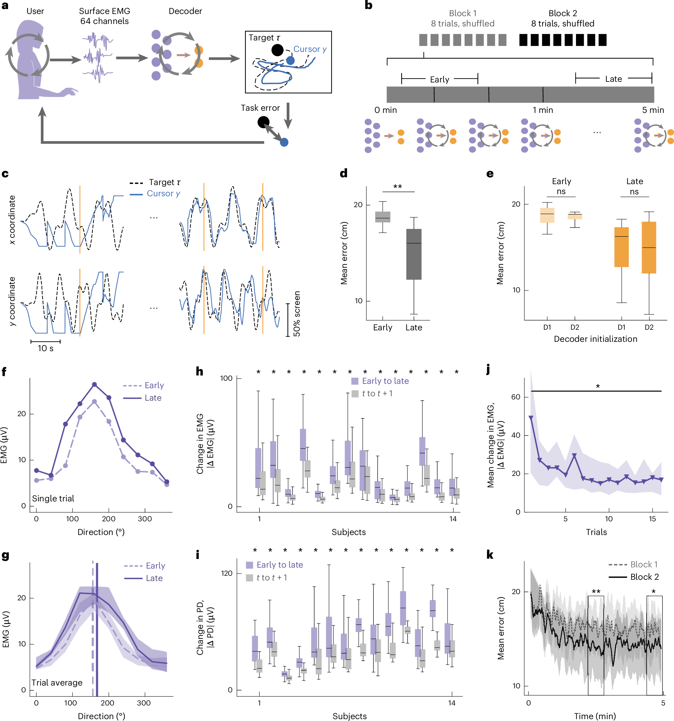
Figure 1. Panel a shows the experiment and feedback loop; b shows the trial structure; c–d show cursor tracking improving over time.
The researchers systematically changed three properties of the decoder: how quickly it updated, how strongly large weights were penalized, and which initial mapping it started with. Those changes let them test whether the computer’s learning rules also changed the human’s learning.
2. Decoder: the algorithm that actually moves the cursor
The Decoder, represented by the matrix D, takes 64 EMG signals and outputs a two-dimensional cursor velocity:
Here, u_t contains the 64 processed muscle-signal values, D has shape 2 × 64, and v_t = (v_x, v_y) tells the cursor how fast to move horizontally and vertically.
For example, one combination of muscle activity may send the cursor to the right, while another sends it upward. Each of the 64 channels contributes according to the current weights in D. The cursor’s position is then updated by integrating this velocity.
How does D learn every 20 seconds?
The online algorithm performs two steps:
- Find a better candidate decoder. Using recent EMG, target positions and cursor positions, it calculates a matrix
D*whose predicted movement points more effectively toward the target. It minimizes a cost with two terms:
The first term compares the decoder’s predicted velocity with the desired corrective movement from the cursor position y toward the target τ. The second term penalizes large decoder weights; λD controls that penalty.
- Blend the candidate with the current decoder. Instead of switching all weights at once, the SmoothBatch update is:
The parameter α is the fraction of the old decoder retained. Thus, α = 0.75 means slow updating and α = 0.25 means fast updating.
Consider just one weight. If its current value is 0.2 and its optimized candidate is 1.0, a slow update changes it to 0.4, while a fast update changes it to 0.8. These numbers are an illustrative calculation using the study’s update rule.
This update is the algorithm that runs during the human experiment. As its matrix changes, the relationship between the participant’s muscles and the cursor changes too.
3. Encoder: how did the researchers measure human learning?
The computer knows D exactly, because it sets those weights. The human’s strategy has to be estimated from behavior.
To do so, the researchers fit another matrix, E, called the user encoder. It predicts the participant’s 64-channel muscle activity from eight task variables:
- Target position: (x,y)
- Target velocity: (v_x,v_y)
- Position error between target and cursor: (e_x,e_y)
- Velocity error between target and cursor:
(velocity error x, y)
In compact form:
The authors estimated E using linear regression on short segments during which D was held fixed. They could then compare E at different moments within a trial.
Suppose the participant initially produces a large EMG response when trying to move right. After practice, the same target direction elicits a different combination or magnitude of muscle activity. That appears as a change in E. D measures the computer’s changing rule; E tracks the person’s changing strategy.
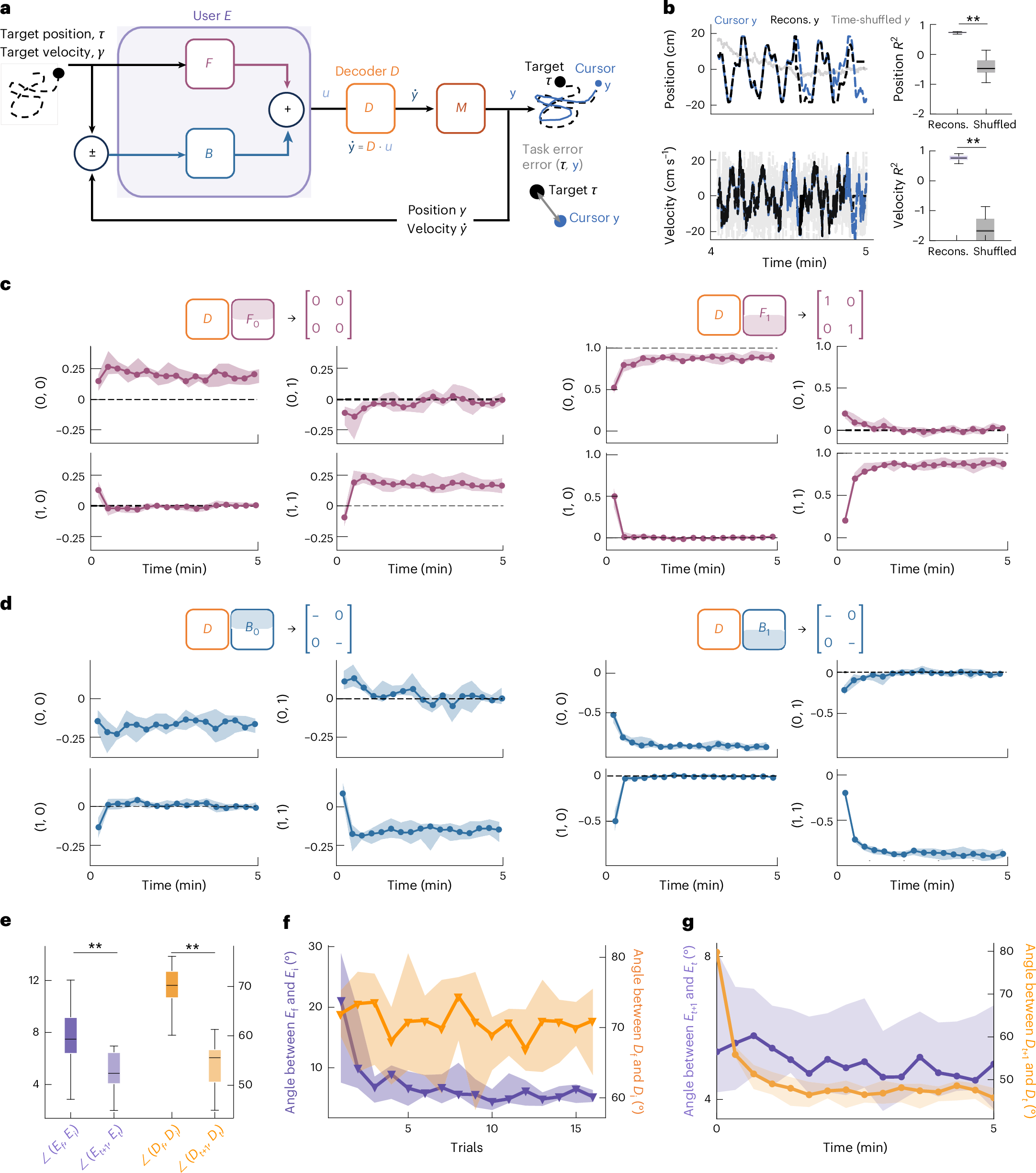
Figure 2. The user encoder links task information to measured EMG. Changes in the estimated encoder describe how a person’s control strategy evolves.
Why examine D and E together?
The actual control loop runs in this order:
Target and visual error → human strategy E → EMG → machine decoder D → cursor → new visual error.
The combined mapping therefore depends on D and E together. In control-theory analysis, the authors separate the encoder into feedforward components (responding to the target trajectory) and feedback components (correcting the cursor’s errors), then examine products such as (DF_1) and (DB_1).
A useful analogy is driving a car with adjustable steering sensitivity. The same steering-wheel turn can produce different vehicle movements after the car’s settings change. How well someone drives depends on both their learned steering strategy and the car’s response.
4. Game theory: what if both sides optimize at once?
Now we have two changing quantities: the human’s E and the machine’s D. The authors built a simplified one-dimensional game in which both learners try to reduce a shared task error, while each also has its own cost for large responses.
A compact potential function captures their trade-off:
(1−DE)²: how well the two mappings work togetherλE × E²: the modeled cost of the user’s control strategyλD × D²: the modeled cost of large decoder weights
For intuition, compare E = 2, D = 0.5 with E = 0.5, D = 2. Both have DE = 1, so the shared-error term is identical. But the work is distributed differently between user and computer. Changing λD changes which combination the system tends toward.
The model also assigns adaptation dynamics to E and D and studies whether they converge to a stable stationary point. Two predictions follow: learning rates affect whether and how fast the pair converges, and changing decoder penalties can change the user’s eventual strategy.

Figure 3. Panel b visualizes the joint optimization landscape; d–e show how learning rates affect convergence; f shows the trade-off between encoder and decoder magnitudes.
5. How did they test those predictions?
The experiment used a 2 × 2 × 2 design: two decoder update speeds, two decoder penalties, and two randomized initializations. That gives eight conditions, each repeated twice per participant.
Test A: fast versus slow decoder updating
The authors compared slow (α = 0.75) with fast (α = 0.25) updates. Participants tracked the target more accurately with the slow-updating decoder, and tracking error decreased more across each trial. Their estimated user encoders also changed more, suggesting that human adaptation proceeded more effectively when the mapping changed gradually.

Figure 4. Panels b–c compare tracking error for fast and slow updates; d compares changes in the user’s encoder; e–f examine the combined control dynamics.
Think of trying to learn a game in which the joystick’s sensitivity changes every few seconds. Updating the rule aggressively might help the computer fit recent data, but it can make the rule harder for the player to learn.
Test B: high versus low decoder penalty
The authors also compared a low penalty (λD = 10²) and a high penalty (λD = 10³). With a stronger penalty, the decoder’s weights became smaller. The estimated user’s encoder magnitude increased: the person compensated for the machine’s weaker response.
Tracking-error improvement remained similar across the two conditions, while cursor speed and individual movement strategies differed. The machine’s objective shaped how the human performed the task, even when overall accuracy was similar.

Figure 5. Panels c–d show the opposing changes in decoder and user-encoder magnitudes; e–g show cursor speed and individual strategies.
The third variable, decoder initialization, was also analyzed: the initial mapping could modestly influence the eventual encoder–decoder relationship.
Takeaway
The study brings together three distinct tools: an online Decoder that controls the cursor, an estimated Encoder that measures human adaptation, and a game-theoretic model that predicts what happens when both change.
Its central finding is that a decoder changes more than cursor accuracy: it changes what the user learns. Better co-adaptive interfaces therefore require designing the interaction between user and algorithm, rather than optimizing the decoder in isolation.
Paper and figures: Madduri, M. M. et al., Nature Machine Intelligence 8, 372–387 (2026). Original article · Data and analysis scripts. Figures 1–5: original authors, CC BY-NC-ND 4.0.
如果你正在学习控制光标,而电脑又不断修改控制规则,会发生什么?
预计阅读时间:约 7–8 分钟。
想象你只能通过收缩前臂肌肉,去控制屏幕上的一个小圆点。你得慢慢摸索:怎样收缩肌肉,光标才会向左、向右或者向上移动?可就在你逐渐找到规律时,电脑还在改变肌肉信号与光标移动之间的对应关系。
这叫 共适应(Co-adaptation):人学习怎样控制机器,机器学习怎样解释人的信号。Madduri 等人通过一个很具体的肌电光标实验,测量两边的变化,再用控制理论和博弈论解释两边为什么会互相影响。
1. 受试者到底做了什么实验?
实验招募了 14 名参与者,在每个人优势侧前臂佩戴 64 通道表面肌电(EMG)电极阵列。屏幕上有两个圆点:一个不断移动的红色目标,以及需要由肌肉控制的蓝色光标。任务就是让蓝点尽可能跟上红点,而红点按照不可预测的二维轨迹移动。
每人完成 16 次实验,每次 5 分钟,分成两个 Block。每次开始时,电脑随机初始化一套肌肉到光标的映射;运行期间,电脑被设定为约每 20 秒更新一次这套规则。
受试者看到光标偏离目标,就尝试换一种肌肉收缩方式。与此同时,电脑也会根据刚刚积累的数据更新映射。这是整篇论文的实验核心:双方都在学习,却又不断改变彼此的学习环境。
Figure 1。a 是实验装置与视觉反馈回路;b 展示实验安排;c–d 显示光标追踪表现随时间改善。
研究者专门操纵了 Decoder 的三个属性:更新速度、权重惩罚和初始权重,看看这些设置能怎样影响人的操作策略。
2. Decoder:电脑真正用来移动光标的算法
实时运行的算法叫 Decoder(解码器),记作矩阵 D。它接收 64 通道肌电信号,计算光标的横向和纵向速度:
这里 u_t 是 64 维肌电信号,(D) 是 2 × 64 的权重矩阵,输出 v_t = (v_x, v_y) 是二维速度。然后电脑把速度按时间累积,更新光标位置。
直观地说,每个肌电通道都会对光标运动产生一定贡献。不同通道的组合经过 D 的加权计算,决定光标往哪里走、走多快。
每 20 秒,Decoder 怎样学习一次?
关键其实只有两步。
第一步:计算一个更好的候选矩阵 D*。 利用最近一段时间的肌电、目标和光标数据,寻找一套能让光标更好地朝目标移动的权重。论文实际优化的是:
把式子拆开看:
D·u:目前这套 Decoder 预测的光标速度。(τ − y)/Δt:从当前光标位置y朝目标τ移动所需的修正速度。- 第一项:希望光标朝目标运动,减少两种速度的差异。
- 第二项:通过
λD惩罚过大的权重,让 Decoder 不必用很大的放大系数才能工作。
第二步:新旧矩阵混合(SmoothBatch)。 作者没有直接把全部权重换成 D*,而是采用:
α 表示旧权重保留多少。所以:
- 慢速更新:
α = 0.75,旧权重保留 75%。 - 快速更新:
α = 0.25,旧权重只保留 25%。
举个数字例子:某个权重原本是 0.2,优化得到的新权重是 1.0。慢速更新后变成 0.4,快速更新后变成 0.8。这只是用论文公式做的计算示例。
理解了这个过程,你就理解了电脑实际运行的学习算法:每隔一段时间,先求一个更合适的 D,再决定多大程度地替换旧 D。
3. Encoder:作者怎样知道人也在学习?
Decoder 的权重 D 是电脑自己设置的,当然可以直接读取。但人的大脑没有给研究者提供一个现成的“肌肉控制策略矩阵”。
因此作者又定义一个 Encoder(编码器)E,根据实际数据去估计:在特定任务情景下,人会产生怎样的肌肉活动?
他们假设肌电活动可以由四组二维信息预测:
- 目标位置:目标的 x、y 坐标。
- 目标速度:目标正在往哪个方向、多快地移动。
- 位置误差:光标离目标多远、偏向哪边。
- 速度误差:光标与目标的运动速度差多少。
总共有 8 个输入维度,用一个 64 × 8 的线性矩阵 E 预测 64 通道 EMG:
作者在 Decoder 固定的短时间区间内,利用线性回归从真实实验数据估计 E,并比较不同时间的 E。
例如,参与者最初想让光标向右时,可能会产生一组很强的肌电;训练后,他可能学会换一组肌肉配合、以不同幅度发力。这些变化就会体现在估计的 E 上。
所以两个字母各司其职:
- D: 电脑实时使用、持续更新的肌电→光标规则。
- E: 研究者从数据中估计、用来追踪人怎样改变策略的模型。
Figure 2。通过任务信息与实测肌电拟合用户 Encoder,再用不同时段的 E 描述操作策略如何变化。
为什么控制理论要把 D 和 E 一起分析?
实际控制链条是:
目标和视觉误差 → 人的策略 E → 64 通道 EMG → 机器 Decoder D → 光标 → 新的视觉误差。
因此系统表现取决于 E 和 D 的共同作用。作者进一步把人的 Encoder 拆成两部分:前馈(Feedforward)负责跟随目标轨迹,反馈(Feedback)负责看到偏差后修正动作,再研究 (DF_1)、(DB_1) 等组合与轨迹追踪和闭环稳定性的关系。
你可以把它想成一辆方向盘灵敏度会变的汽车。司机有自己的转向习惯,汽车有自己的响应规律。驾驶体验取决于两者能否配合;光研究方向盘本身还不够。
4. 博弈论:人和电脑都在优化,会走向什么状态?
到这里,我们已经有两个会变化的对象:人的 E 和电脑的 D。作者于是构建一个简化的一维博弈论模型,假设双方都希望追踪得更准确,同时各自会受到“控制幅度成本”的影响。
论文中的势函数(Potential Function)可以写成:
理解三个部分就够了:
(1−DE)²:衡量人和电脑配合后的任务误差。λE × E²:人的控制策略在模型中的成本。λD × D²:电脑使用较大 Decoder 权重的成本。
例如两个组合:E = 2、D = 0.5,或者 E = 0.5、D = 2。它们都有 DE = 1,任务误差项完全相同,但一个需要更大的 E,另一个需要更大的 D。
那么该选哪一个?就取决于模型给人和机器分别设定的成本权重 λE、λD。
作者进一步建立两边同时调整的动态模型,观察 E 和 D 能否收敛到稳定状态(Stationary Point),并预测出两个重要关系:
第一,双方的学习速度会共同影响收敛。第二,改变机器的惩罚系数,也会改变人最终形成的策略。
Figure 3。b 展示联合优化的势函数地形;d–e 研究学习率与收敛;f 展示 Encoder、Decoder 幅度的相互补偿。
5. 作者究竟比较了哪些实验条件?
实验使用一个 2 × 2 × 2 设计:两种学习速度、两种权重惩罚、两种随机初始化。一共 8 种 Decoder 条件,每个参与者将这八种条件各做两次,所以总计 16 次试验。
实验 A:Decoder 更新得越快越好吗?
作者比较:
- 慢速更新:
α = 0.75 - 快速更新:
α = 0.25
结果是慢速组的光标追踪误差更小,而且每次 5 分钟实验中改善得更多。研究者估计的用户 Encoder 也在慢速条件下变化得更多,说明人的控制策略能够更充分地逐渐调整。
Figure 4。b–c 比较快慢更新下的追踪误差;d 比较用户 Encoder 的变化;e–f 分析双方组合起来的追踪和稳定性。
可以类比你在学习操作游戏手柄:如果摇杆灵敏度总是大幅改变,就算每次调整对机器来说有道理,玩家也很难建立稳定的操作习惯。
实验 B:改变 Decoder 的惩罚项,会发生什么?
作者比较:
- 低惩罚:
λD = 10² - 高惩罚:
λD = 10³
惩罚越大,优化算法越倾向于降低 Decoder 权重的幅度。实验发现:当 D 变小时,估计的人体 Encoder 幅度反而增大——参与者调整了肌肉控制策略,补偿机器响应幅度的变化。
两种设置下,追踪误差的改善程度相近,但光标运动速度和参与者采取的控制策略不同。机器改变了人的操作方式,即使最终追踪成绩看起来差不多。
Figure 5。c–d 展示机器 D 与用户 E 的幅度变化;e 展示光标速度;f–g 展示不同参与者各自的补偿策略。
作者还比较了两种随机初始化方式,发现初始映射也可能对后续双方形成的控制关系产生一定影响。
总结
这篇论文最容易理解的方式,是把它拆成三个独立工具:
Decoder D 是实时算法,真正把 EMG 转成光标移动,并通过 SmoothBatch 不断更新;Encoder E 是研究者拟合的人体行为模型,用来观察人的控制策略如何变化;博弈论则负责解释和预测,当人和机器都在调整时,系统会朝什么状态发展。
最重要的发现是:Decoder 不只决定当前控制得准不准,还会影响人最终学会怎样控制。 设计闭环神经接口,本质上是在设计两套学习过程之间的互动。
论文与图片: Madduri, M. M. et al., Nature Machine Intelligence 8, 372–387 (2026)。原论文 · 数据与分析代码。配图来自论文 Figures 1–5,原作者署名,CC BY-NC-ND 4.0。