
readApaper#5 Engineering Neuronal Network Connectivity Through Precise and Scalable Electrical Modulation
Can we train living neuronal networks by tuning their connections, the way we train artificial neural networks?
Reading time: about 7–8 minutes
Artificial neural networks learn by updating connection weights. But what if we try to do something similar with actual neurons? Could we pick two locations in a living network, strengthen the influence of one on the other, and then show that the change persists after stimulation has stopped?
That last question is harder than it sounds. Making a neuron fire is not the same as changing how a network is wired.
In a 2026 paper in Advanced Science, Sreedhar S. Kumar and colleagues combined high-density microelectrode arrays (HD-MEAs), spike-timing-dependent plasticity (STDP), and a new readout called Conditional Activity Metrics (CAM). Their goal was to make neuronal circuit shaping more targeted, measurable, and scalable.
The framework has three essential steps: read the network, stimulate candidate connections, and verify what changed.
1. What is a biological “weight”?
In a conventional neural network, a weight w represents how strongly one unit influences another. A biological excitatory synapse plays a roughly analogous role, but its efficacy cannot be set by simply assigning a number.
Suppose neuron A connects to neuron B. When A generates an action potential (AP), the signal travels along its axon and triggers neurotransmitter release. This can depolarize B, producing an excitatory postsynaptic potential (EPSP).
An EPSP is not itself an action potential. It is one contribution toward B reaching its firing threshold. If A→B becomes more effective, the same input from A may produce a larger EPSP, making B more likely to fire.
This capacity for activity-dependent change is called synaptic plasticity. It is a major component of biological learning, but unlike an artificial model’s weight matrix, it involves receptors, release probability, excitability, and many other cellular processes.
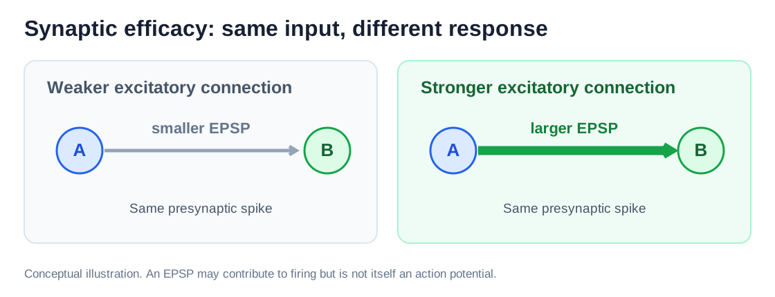
Figure 1. Original explanatory schematic (English labels): a stronger excitatory pathway can produce a larger postsynaptic effect from the same presynaptic input. This is not a directly measured weight map; compare the study’s conceptual Figure 1a–c.
2. Can spike timing train a connection?
A classic rule of plasticity is spike-timing-dependent plasticity, or STDP. The order of two spikes matters.
For a typical excitatory STDP relationship:
- Pre → Post: the presynaptic neuron fires shortly before the postsynaptic neuron. This timing often favors long-term potentiation (LTP).
- Post → Pre: the postsynaptic neuron fires first. This timing often favors long-term depression (LTD).
For example, imagine A firing at 0 ms and B firing at +5 ms. Repeating this pairing may strengthen A→B in suitable biological conditions. The reverse order may favor weakening.
This is not a universal rule: cell type, network activity, and stimulation parameters can reverse or eliminate the expected effect. Still, STDP suggests a testable engineering strategy: impose a carefully chosen stimulation sequence instead of waiting for that sequence to occur by chance.
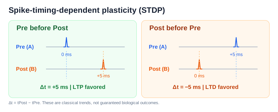
Figure 2. Original schematic of a classical excitatory STDP rule. We define Δt = tPost − tPre. The arrows show tendencies, not guaranteed outcomes.
Implementing the idea with an HD-MEA
An HD-MEA is a silicon chip covered in tiny electrodes. Neurons or slices placed on the chip generate extracellular electrical signals that the electrodes can record; selected electrodes can also deliver programmed pulses.
The main device in this study provides 26,400 addressable electrodes, spaced 17.5 μm apart, with up to 1,024 simultaneous recording channels (typically sampled at 20 kHz).
The experiment follows a practical sequence:
- Record baseline activity. Collect spontaneous spike trains and find where the network is active.
- Select candidate pairs. Look for electrodes whose spike trains show consistent temporal relationships. These are putative functional connections, not necessarily proven single synapses.
- Deliver paired stimulation. Apply one biphasic pulse at a candidate presynaptic electrode, followed after a controlled delay by a burst of 5–10 pulses at the postsynaptic site. Repeating the sequence attempts to induce plasticity.
- Record again. After stimulation, ask whether the relationship between the two sites has changed.
A crucial distinction: accurately timed electrical stimulation commands do not guarantee equally precise neuronal spikes. The authors therefore also evaluated response reliability and stimulation artifacts.
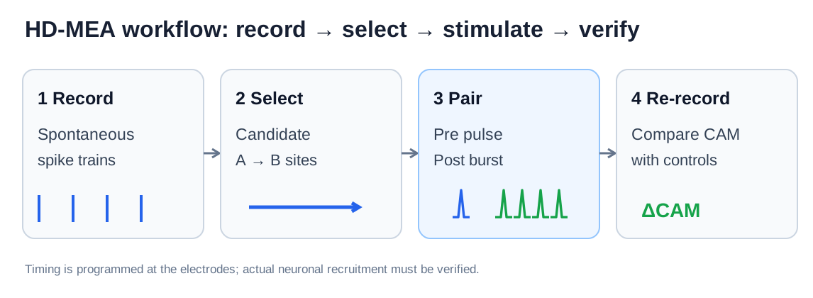
Figure 3. Original workflow schematic, adapted conceptually from the paper’s Figure 1g. It separates observing a candidate relationship, delivering stimulation, and evaluating the response.
3. Did the synapse really become stronger?
Stimulating A and observing more spikes at B would not, by itself, prove that A→B had strengthened. B might simply have become more excitable, or the whole network might have entered a more active state.
The authors therefore used two complementary kinds of evidence.
Direct electrophysiological evidence: patch clamp
A patch-clamp electrode can record the membrane voltage of a particular postsynaptic neuron. In a selected rat cortical culture, the researchers identified a stimulation site that consistently elicited an EPSP in the patched neuron.
They then delivered 100 STDP pairings. Afterward, when they stimulated the candidate presynaptic site again, the mean EPSP amplitude was approximately 20% greater than before, with a statistically significant difference.
That is stronger evidence than an increase in spike counts alone: the postsynaptic membrane response to a comparable test input became larger.
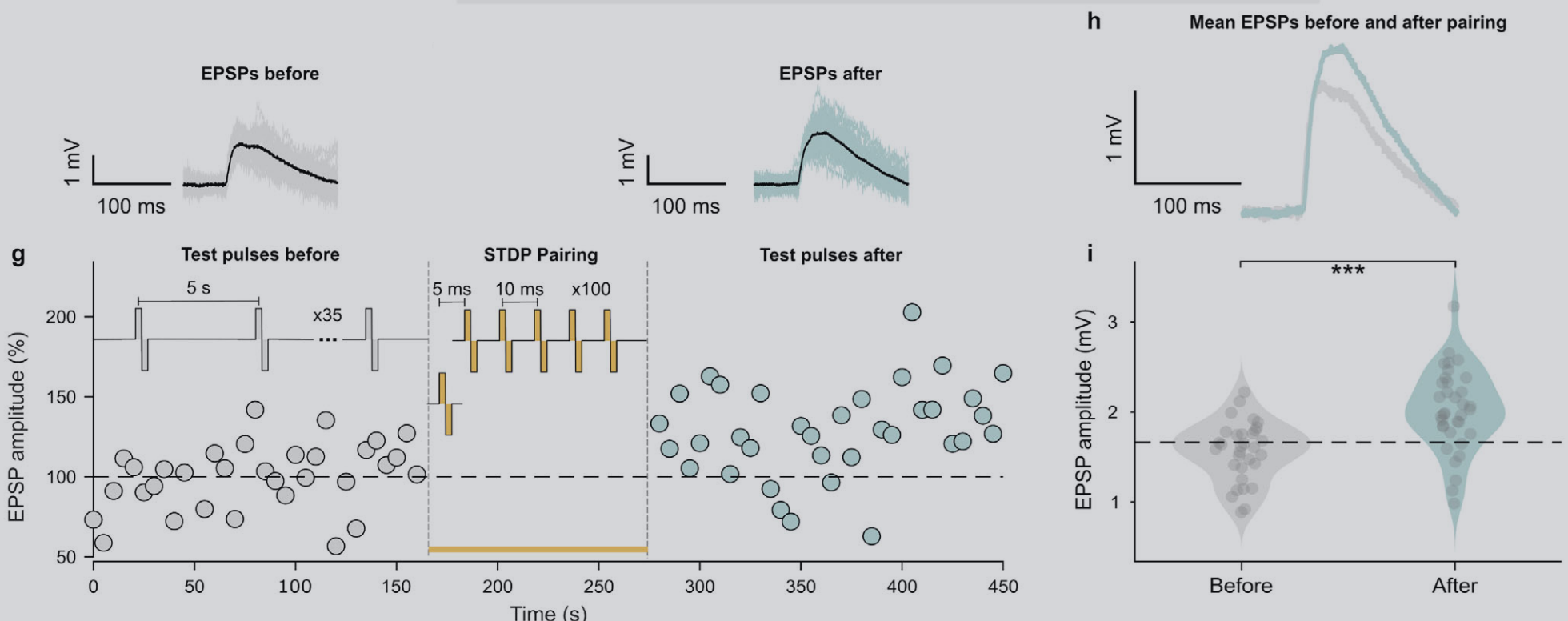
Figure 4. Original experimental Figure 2g–i from Kumar et al. (2026). Panel g tracks normalized EPSP amplitudes before and after pairing; h compares the mean EPSP waveforms (about 20% enhancement in this example); i shows the amplitude distributions and statistical test (p < 0.001). These are results from selected recordings—not a 20% improvement for every connection. View the figure at the publisher.
Patch clamp is convincing, but it is difficult to apply to hundreds of cells at once. That motivates a scalable readout from extracellular spike trains.
4. CAM: measuring change without directly reading synaptic weights
The authors introduce Conditional Activity Metrics (CAM). Rather than asking how often B fires overall, CAM asks:
Given that A just fired, what happens next at B?
Imagine observing B for 50 ms after each spike from A. In a simplified example:
| Measure | Before | After |
|---|---|---|
| First spike from B | 20 ms after A | 8 ms after A |
| Spikes from B within 50 ms | 2 | 4 |
These numbers are illustrative, not measurements from the paper.
Two aspects have changed:
- First-spike latency, t₁: B tends to respond earlier after A’s spike.
- Conditional spike density, ρ: B produces more spikes in the designated post-spike window.
CAM combines these into a two-dimensional metric, CAM = (t₁, ρ). In the actual analysis, it aggregates many presynaptic spike events; the windows for measuring latency and density need not be identical.
For a strengthening-like change, we might observe Δt₁ < 0** and **Δρ > 0. The opposite pattern can be consistent with weakening.
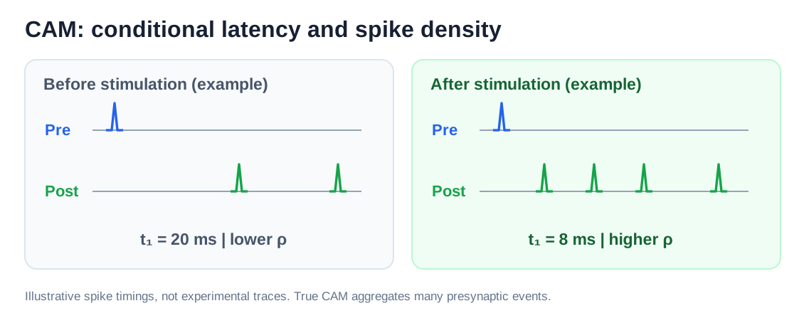
Figure 5. Original schematic using hypothetical spike times: CAM summarizes when B first responds and how densely B fires after A. It is not a direct measurement of one synaptic weight.
Why control pairs matter
What if every neuron starts firing more frequently after stimulation? A change in CAM for one pair would then be much less persuasive.
The authors compare each target pair’s change in CAM (ΔCAM) with a distribution of changes from matched control pairs in the same network. A robust Mahalanobis distance measures how far the target change lies from normal network variation, accounting for the joint variability of latency and density.
In plain terms: a change only counts as compelling evidence of targeted circuit shaping when it stands out from the controls.
Can CAM track known weights?
To evaluate the metric under controlled conditions, the researchers used a simulated 2,000-neuron spiking network and explicitly modified selected synaptic weights.
The reported correlations were strong:
- Weight change vs. density change: r = +0.93.
- Weight change vs. latency change: r = −0.91.
Those numbers come from simulation, where the modified weight is known. They do not imply that the real weight of any biological synapse can be uniquely reconstructed from CAM.
The experimental CAM values were measured mainly at the electrode / multi-unit-activity level, where several neurons may contribute to one channel. They therefore reflect changes in local functional relationships, not exact weights of isolated synapses.
5. What worked in living tissue?
The authors tested the framework in three preparations:
- Dissociated rat cortical neuron cultures, which provide long-term access to developing networks.
- Acute mouse cortical slices, which retain some native local circuitry.
- Mouse stem-cell-derived cerebral organoid slices, which offer a more complex tissue-like environment.
In the 2D cultures, 87 of 227 tested electrode pairs (38.3%) showed statistically significant CAM changes. In the slice and organoid preparations combined, 20 of 52 pairs (38.5%) were significant.
Across all experiments, that is 107 of 279 pairs—roughly 40%.
The team also demonstrated parallel stimulation, using as many as eight stimulation sites. In a subset followed for longer periods, the induced effects persisted for at least 90 minutes.
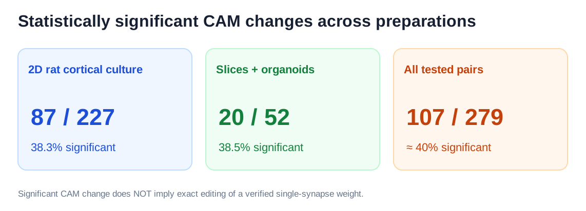
Figure 6. Original data-summary visualization using counts reported in the paper. “Significant” refers to detected CAM changes—not successful editing of a known single-synapse weight to a prescribed value.
This distinction matters. Some pairs did not change significantly, and some changed in a direction that did not match the simple STDP prediction. The result is an encouraging demonstration of scalability, not a fully predictable biological weight-editing machine.
6. Is this already a trainable biological computer?
Not yet. But the work assembles three capabilities a future system would need:
Read: observe the network and identify candidate functional connections.
Write: deliver precisely timed stimulation intended to reshape those connections.
Verify: measure whether the functional relationship changes after the intervention, and compare the result with controls.
A genuinely task-driven biohybrid computer would also need an input encoding, an output decoder, a task objective, and a feedback strategy that adjusts future stimulation according to performance.
This paper does not demonstrate autonomous task learning in an organoid. It addresses a narrower—and very important—engineering problem: making circuit changes measurable and, to a degree, targetable.
Takeaway
The central advance is not a new law of neuroplasticity. It is an integrated HD-MEA + STDP + CAM workflow that moves beyond merely observing spikes or provoking transient activity.
We are still far from assigning arbitrary weights to living neurons as we do in software. But learning to read, perturb, and verify functional connections is a meaningful step toward more systematic neural-circuit training.
Paper: Sreedhar S. Kumar et al., Engineering Neuronal Network Connectivity Through Precise and Scalable Electrical Modulation, Advanced Science (2026). DOI: 10.1002/advs.75473.
Figures: Original diagrams (1, 2, 3, 5, 6) created for this article; experimental Figure 4 reproduced from Kumar et al., Figure 2g–i. Original paper licensed under CC BY; image credits remain with the authors.
我们能像训练人工神经网络一样,训练真实的神经元吗?
目标阅读时间:约 7–8 分钟
我们知道,人工神经网络通过不断调整神经元之间的连接权重来学习。如果将这个想法应用于真实的生物神经网络呢?
假设培养皿中有几千个神经元,我们能否指定其中两个神经元,让它们之间的连接变强?甚至让另一些连接变弱?
更重要的是:改变之后,我们怎么知道网络真的发生了变化,而不是仅仅因为电刺激暂时兴奋了起来?
2026 年,来自 ETH Zurich 等机构的研究团队在 Advanced Science 上发表了一项研究,试图解决这个问题。他们结合高密度微电极阵列(HD-MEA)、脉冲时序依赖可塑性(STDP)和一种新的神经活动指标(CAM),实现了对生物神经网络中部分功能连接的定向调控与验证。
这篇论文的真正价值,不只是能够刺激神经元,而是尝试建立一套读取连接、改变连接、验证连接的完整技术框架。
1. 生物神经网络中的“权重”是什么?
在人工神经网络中,我们通常使用权重 w 表示一个神经元对另一个神经元的影响程度。生物神经网络也有类似现象。
假设两个神经元 A 和 B 通过一个兴奋性突触连接。当 A 产生动作电位(Action Potential,AP)时,信号沿轴突传递,引起突触前末端释放神经递质,进而改变 B 的膜电位。
如果这种输入是兴奋性的,B 的膜电位可能短暂上升,形成一个兴奋性突触后电位(EPSP)。但 EPSP 不等于动作电位:B 需要达到相应的放电阈值,才可能产生新的动作电位。
如果 A→B 的突触效能增强,同样的 A 输入就可能在 B 上产生更大的 EPSP,使 B 更容易被激活。这就是突触可塑性(Synaptic Plasticity)的一个重要表现。
你可以把突触权重理解为一条连接传递信息的有效程度。不过,与人工神经网络不同,真实突触的强度受到神经递质释放、受体状态和细胞自身兴奋性等多种因素影响,并不是一个可以直接赋值的数字。
因此,生物神经网络的训练,不能简单地通过修改一个权重矩阵来实现。研究人员需要利用神经元自身的可塑性机制。
配图 1|自绘概念示意:相同的突触前输入在较强连接下可能诱发更大的突触后电位(EPSP)。原论文完整回路塑形构想参见 Figure 1a–c。
2. 如何让两个神经元之间的连接变强?
这里需要了解一个经典机制:STDP(Spike-Timing-Dependent Plasticity,脉冲时序依赖可塑性)。
它的核心是:神经元放电的先后顺序,可能影响突触效能的变化方向。
对于经典的兴奋性 STDP:
- Pre → Post: 突触前神经元先放电,突触后神经元紧接着放电,通常偏向诱导长时程增强(LTP)。
- Post → Pre: 突触后神经元先放电,随后突触前神经元才放电,通常偏向诱导长时程抑制(LTD)。
例如 A 在 0 ms 放电,B 在 5 ms 放电。如果这种时间关系反复出现,在适当的生物条件下,A→B 的连接就可能增强。
这并不是神经元有意识地判断“A 导致了 B 放电”,而是精确的活动时序会触发细胞内部的可塑性机制。STDP 也不是任何神经元都遵循的固定规则;它的方向和幅度还受到神经元类型、网络状态及刺激参数影响。
关键的问题是:能否人为控制两个位置的放电时序?
把 STDP 变成实际实验
作者使用了 HD-MEA(High-Density Microelectrode Array,高密度微电极阵列):一块布满微小电极的芯片。神经元位于电极上方,电极既能记录细胞外活动,也能向指定位置施加电脉冲。
本文的主要芯片拥有 26,400 个电极位置,电极间距 17.5 μm,最多支持 1,024 个通道同时记录,主要采样率为 20 kHz。
实验流程为:
- 记录自发活动: 先观察约 15–45 分钟的 Spike Train(脉冲序列),建立刺激前的活动基线。
- 选择候选连接: 利用放电时间关系与互相关等分析,筛选可能存在功能联系的电极配对。
- 施加配对刺激: 在候选 Pre 位置施加一个双相电脉冲,短暂延迟后在 Post 位置施加由 5–10 个脉冲构成的 Burst;改变前后顺序则尝试诱导相反的可塑性。
- 停止刺激后再记录: 检查目标位置之间的活动关系是否保留了可检测的变化。
这里需要区分电刺激指令的时序和神经元实际动作电位的时序:前者可以被精确设置,后者还取决于刺激能否可靠地激活目标细胞。
配图 2|自绘 SVG 示意:经典兴奋性 STDP 的正延迟和负延迟。Δt=tPost−tPre,箭头表示统计意义上的典型塑性方向,并非必然结果。
配图 3|自绘 SVG 示意:HD-MEA 的记录、配对刺激与后续 CAM 评估流程;参考原论文 Figure 1g。
3. 刺激成功,是否就意味着连接增强?
并不一定。
首先,电极发出电脉冲不代表目标神经元每次都能成功产生 AP。其次,就算刺激之后 B 放电更多,也可能是整个网络的兴奋性提高,而非 A→B 连接特异性增强。
作者因此采用两个层次的验证。
直接电生理验证:观察 EPSP
研究人员通过同步 HD-MEA 与膜片钳(Patch-clamp)记录,在选定实验中观察刺激 A 是否能够在 B 上诱发 EPSP。
在一个代表性实验中,他们找到能够引起目标神经元 B 的 EPSP 的候选突触前刺激位置 A,随后进行 100 次配对刺激。训练结束后,再以相同类型的测试脉冲刺激 A。
结果发现,**B 的平均 EPSP 振幅增加约 20%**,差异具有统计显著性。这为该刺激方法确实能够增强突触传递效能提供了直接的电生理证据。
但膜片钳非常依赖精细的单细胞操作,难以大规模并行验证。因此作者还需要一种能直接从 HD-MEA Spike Train 计算的反馈指标。
图 4|原论文 Figure 2g–i:同步 HD-MEA 与膜片钳记录验证配对刺激后的突触效能增强。(g) 配对刺激前后,测试脉冲诱发的 EPSP 归一化振幅随时间的变化;(h) 训练前后平均 EPSP 波形对比,训练后平均振幅增加约 20%;(i) EPSP 振幅分布与统计检验(p < 0.001)。这些数据来自选定的代表性实验,不能理解为所有连接都会增强 20%。来源:Kumar et al., Advanced Science (2026), Figure 2g–i,原图截图。查看论文原图。
4. CAM:不直接测突触权重,怎么知道连接变了?
作者提出了 CAM(Conditional Activity Metrics,条件活动指标)。
想象每次 A 放电后,我们观察 B 在接下来 50 ms 内的活动。假设出现下面的情况:
| 指标 | 刺激前 | 刺激后 |
|---|---|---|
| B 的首次放电时间 | A 放电后 20 ms | A 放电后 8 ms |
| 50 ms 内 B 的放电次数 | 2 次 | 4 次 |
以上为帮助理解的假想数据,并非论文实际测量值。
刺激后,B 的反应有两个变化:更早,而且更频繁。
CAM 正是用两个分量捕捉这些信息:
- t₁: A 放电之后,B 首次放电延迟的条件中位数。
- ρ: A 放电之后的特定时间窗口内,B 的平均条件放电密度。
它们合在一起,形成一个二维活动关系指标。实际计算聚合了大量 A 的 Spike 事件,两类指标的时间窗口也可以不同。
连接增强时,典型方向是 Δt₁ < 0、Δρ > 0,即首次放电延迟缩短、条件放电密度增加。减弱时可能观察到相反变化。
为什么一定要设置对照组?
因为 CAM 发生变化,不等于特定连接必然改变。
如果整个网络更兴奋,目标电极上的 Spike 活动也可能发生变化。作者因此从同一个网络中选择其他对照电极对,比较刺激前后 CAM 的变化。
真正关心的问题是:
目标配对的变化,是否明显超出了其他配对的正常波动?
作者使用稳健马氏距离(Robust Mahalanobis Distance)等方法,衡量目标配对的 ΔCAM 相对于对照分布是否显著偏离。
这个方法靠谱吗?
作者先构建了一个 2,000 神经元的脉冲神经网络(SNN)。因为仿真中可以直接指定突触权重,所以能够人为改变已知连接,并检验 CAM 是否反映改变。
结果显示:
- 突触权重变化与 Δρ 的相关系数为 r = 0.93;
- 与 Δt₁ 的相关系数为 r = −0.91。
说明在作者的仿真设置中,CAM 对已知的权重变化有较强敏感性。
但需要强调:CAM 不是直接测量单个真实突触的权重。真实电极可能混合记录多个神经元的活动,网络结构与共同输入也会影响条件放电关系。
配图 5|自绘 SVG 示例:CAM 从多个 Pre Spike 后的 Post 条件放电中提取首次延迟 t₁ 与密度 ρ。图中的 20 ms、8 ms 等为示例值;论文的仿真验证详见 Figure 3c–e。
5. 真实生物网络中的结果如何?
完成方法验证后,作者将其应用于不同的真实神经组织模型。
二维大鼠皮层神经元培养物
在 227 对测试电极配对中,有 87 对(38.3%) 出现了统计显著的 CAM 变化。代表性实验中,正延迟配对刺激与更短的延迟、更高的条件放电密度一致,负延迟协议则出现相反方向的变化。
作者还进行了并行刺激:在同一芯片上最多同时刺激 8 个位置;高通量模式下测试的 89 对中,37 对出现显著变化。
脑切片与脑类器官
作者随后在小鼠急性皮层切片、以及小鼠干细胞来源的脑类器官切片中进行了实验。这些组织保留了更复杂的空间结构和局部回路。
两类组织合计测试 52 对电极,20 对(38.5%)出现显著变化。脑类器官的代表性实验中,+7 ms 和 −7 ms 配对刺激后出现了符合增强、减弱方向的不同 CAM 位移。
合计来看,279 对电极配对中约 40% 出现统计显著的可塑性相关活动变化。部分长期追踪的配对,效应至少持续 90 分钟。
不过,40% 并不意味着研究人员能按指定方向精确编辑 40% 的真实单突触。还有配对没有显著反应,甚至出现与经典 STDP 预测相反的变化。
配图 6|自绘统计摘要:二维神经元培养网络与脑切片/类器官模型中,发生显著 CAM 改变的电极对数量。来源:原论文 Figure S4、Figure 5–6 及 Results。
6. 这是否意味着我们可以训练“生物计算机”?
还没有,但这项研究提供了重要基础。
作者把三种能力组合起来:
Read(读取):记录神经活动,识别候选功能连接。
Write(写入):通过精确的时序电刺激诱导塑性。
Verify(验证):用 CAM 与对照统计,检查局部活动关系是否持续改变。
在人工神经网络中,算法能直接修改权重。真实神经网络则必须通过细胞自身的机制产生变化,而且结果存在显著异质性。
本研究还存在明确的边界:
- 不同电极对对刺激的响应不一致,连接变化方向并不总能预测;
- 电极刺激可能影响多个局部神经元,CAM 也是间接测量;
- 论文没有建立根据任务表现自动更新刺激策略、训练脑类器官完成复杂任务的完整闭环系统。
未来可以探索根据 CAM 等反馈指标,自动调整刺激位置、延迟和强度,让“回路塑形”逐步发展为任务驱动的神经网络训练。
结语
这篇论文的重要性不在于发现一种新的学习规律,而在于将已有的 STDP 原理、HD-MEA 硬件和可扩展的神经活动分析方法结合成了一套回路塑形技术。
过去,我们可以观察神经网络,也可以通过刺激短暂干预它们。现在,研究人员正在尝试更进一步:有选择地改变真实神经网络的连接,并在刺激结束后验证这些改变是否持续存在。
距离像训练人工神经网络那样精准地训练生物神经网络,仍然有很长的路要走。但从被动记录迈向主动塑形,这是一项值得关注的进展。
论文信息
- Title: Engineering Neuronal Network Connectivity Through Precise and Scalable Electrical Modulation
- Authors: Sreedhar S. Kumar et al.
- Journal: Advanced Science (2026)
- DOI: 10.1002/advs.75473
- 图片授权: 原论文 CC BY;正式使用时保留原图 Figure 编号、出处及改动说明。