readApaper#11 The Neural Hawkes Process: A Neurally Self-Modulating Multivariate Point Process

Reading time: about 6–7 minutes · 2026-10-28 · NeurIPS 2017

Why does one event make another more likely—and why can that influence change several times before the next event even occurs?

Mei and Eisner’s Neural Hawkes Process offers a way to learn the timing and types of events from their history. The key idea is to couple a continuous-time LSTM with a temporal point process: the LSTM remembers what happened, while the point process predicts when the next event will happen and what kind of event it will be. The memory changes when an event arrives and keeps evolving during the quiet intervals between events.

1. Start with Hawkes: the past changes the future

Imagine observing neurons A and B. A fires at 10 ms; B fires at 14 ms. Does A’s firing make B more likely to fire next? Does that effect disappear after a few milliseconds?

A classical Hawkes process describes precisely this kind of history dependence. Every event type has a time-varying intensity, $\lambda_k(t)$, meaning its instantaneous expected event rate. Within a very short interval $dt$, the probability of an event of type $k$ is approximately $\lambda_k(t)\,dt$.

In the classical exponentially decaying version,

$$\lambda_k(t)=\mu_k+\sum_{t_j<t}\alpha_{k_j,k}\exp[-\delta_{k_j,k}(t-t_j)].$$

The baseline $\mu_k$ is the background event rate. Each past event adds an influence of size $\alpha$, which fades with decay rate $\delta$. In the standard self-exciting Hawkes process, those added influences are positive.

This works nicely for simple excitation, but some event sequences are more intricate. An event may inhibit another event; repeated events may produce diminishing returns; the effects may depend on the order of earlier events; and an effect may appear only after a delay. Neural Hawkes learns such patterns from the sequence rather than insisting on one fixed additive rule.

2. The key innovation: an LSTM that also changes between events

An ordinary LSTM updates its state as new inputs arrive. The paper designs a continuous-time LSTM (CT-LSTM) with two complementary operations.

When event $i$ occurs: the event type and the preceding state pass through LSTM-like gates. They determine a new memory value $c_i$, a target memory $\bar c_i$, and a positive decay-rate vector $\delta_i$.

While no new event occurs: every memory component follows a continuous curve:

$$c(t)=\bar c_i+(c_i-\bar c_i)\odot\exp[-\delta_i(t-t_i)], \quad t_i<t\leq t_{i+1}.$$

The formula is intuitive. Immediately after an event, memory starts at $c_i$. As time passes, it approaches $\bar c_i$. The learned $\delta_i$ decides how quickly that happens. Because these are vectors, some dimensions can remember very recent events while others carry longer-lived context.

The target memory matters: the state is relaxing toward a learned, history-dependent value, not necessarily toward zero. The interval without events therefore carries information too—the model’s state keeps changing as time passes.

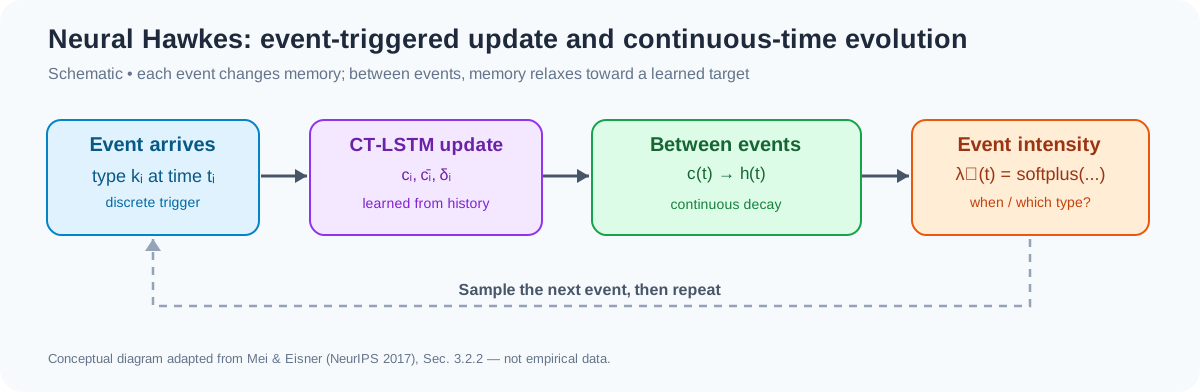
Schematic of the continuous-time loop. Each event updates the CT-LSTM, which determines the memory dynamics between events; the resulting intensities govern the next event. Self-drawn from the mechanism in Section 3.2.2.

In the original paper’s Figure 1, the purple and green intensity curves show how the same event can excite one event type but inhibit another. The curves can jump when an event occurs, then change continuously afterward. See original Figure 1 in the paper.

3. Turning continuous memory into future-event predictions

The changing cell memory is converted to a hidden state $h(t)$ by an output gate and a nonlinear function. Then each event type receives its own intensity:

$$\lambda_k(t)=f_k\!\left(w_k^\top h(t)\right), \qquad f_k(x)=s_k\log(1+\exp(x/s_k)).$$

The scaled softplus function keeps the intensity positive. The weight vector $w_k$ maps the shared history representation to event type $k$; $s_k$ controls the transfer function’s scale.

For neurons, we might interpret the event type as a neuron ID and each event as a spike. The model then assigns every neuron a time-varying firing intensity. In the paper’s experiments, event types instead represent observations such as social-media actions, online phrases, or clinical records.

How is it trained? By maximizing the point-process log-likelihood:

$$\ell=\sum_{i:t_i\leq T}\log\lambda_{k_i}(t_i)-\int_0^T\sum_k\lambda_k(t)\,dt.$$

The first term rewards high intensity where events actually occur. The second measures the total predicted intensity across all the periods in which events could have occurred. Together, they teach the model both the observed event timings and the intervals of silence. The authors approximate the integral with Monte Carlo sampling.

4. What did the experiments show?

The authors compared three models: classical self-exciting Hawkes (SE-MPP), Hawkes with inhibition and nonlinear intensity (D-SM-MPP), and the proposed Neural Hawkes (N-SM-MPP).

On Retweets (three event types) and MemeTrack (5,000 event types), the neural version achieved substantially better test log-likelihood per event. The improvement over D-SM-MPP is particularly informative: adding inhibition helps, but the recurrent representation of complete event history adds further predictive power. See Figure 2 for the learning curves and Figure 3 for the per-sequence comparisons.

The paper also examined synthetic streams and real datasets involving financial activity, MIMIC-II clinical events, and Stack Overflow. In an experiment that systematically hid selected event types, the neural model outperformed classical Hawkes across all 31 evaluated missing-event-type combinations (Figure 4). On next-event prediction, its improvements were especially consistent for event type; results for event time were more mixed.

5. Why does this matter beyond the equations?

Think about a viral post. One retweet may briefly increase the chance of another. Several retweets in quick succession can create a wave of attention. But what if no one retweets it for an hour? That quiet interval also tells us something about what might happen next.

The same principle applies to other event streams, from online discussions to sequences of clinical records. What happened matters, but so do the order of events and the time between them. A model that keeps track of time between observations can use both the events and the gaps to build a better picture of what comes next.

Neural Hawkes makes this possible by giving the past a changing influence: every new event reshapes the model’s memory, and that memory continues to evolve until another event appears.

Takeaway

Neural Hawkes gives event sequences a memory that keeps changing even when nothing happens. Instead of treating the past as a simple collection of fading signals, it learns how different events interact over time. The central lesson is simple: to predict the next event, we need to understand not only what happened, but also when it happened.

---

References / 参考资料

• Mei, H., & Eisner, J. (2017). The Neural Hawkes Process: A Neurally Self-Modulating Multivariate Point Process. Advances in Neural Information Processing Systems, 30. NeurIPS paper · Full PDF.
• Author’s original code (Theano).
• Schematic diagram is original and explanatory, based on the architecture described by Mei & Eisner (2017), Section 3.2.2.